---
title: Monitoring dashboard
enableTableOfContents: true
updatedOn: '2026-01-09T15:13:11.226Z'
---

The **Monitoring** dashboard in the Neon console provides several graphs for monitoring system and database metrics. You can access the **Monitoring** dashboard from the sidebar in the Neon Console. Observable metrics include:

Your Neon plan defines the range of data you can view.

| Neon Plan | Data Access |
| --------- | ----------- |
| Free      | 1 day       |
| Launch    | 3 days      |
| Scale     | 14 days     |

You can select different periods or a custom period within the permitted range from the menu on the dashboard.

The dashboard displays metrics for the selected **Branch** and **Compute**. Use the drop-down menus to view metrics for a different branch or compute. Use the **Refresh** button to update the displayed metrics.

If your compute was idle or there has not been much activity, graphs may display this message: `There is no data to display at the moment`. In this case, try selecting a different time period or returning later after more usage data has been collected.

All time values displayed in graphs are in [Coordinated Universal Time (UTC)](https://en.wikipedia.org/wiki/Coordinated_Universal_Time).

<Admonition type="note" title="Endpoint Inactive: What does it mean?">
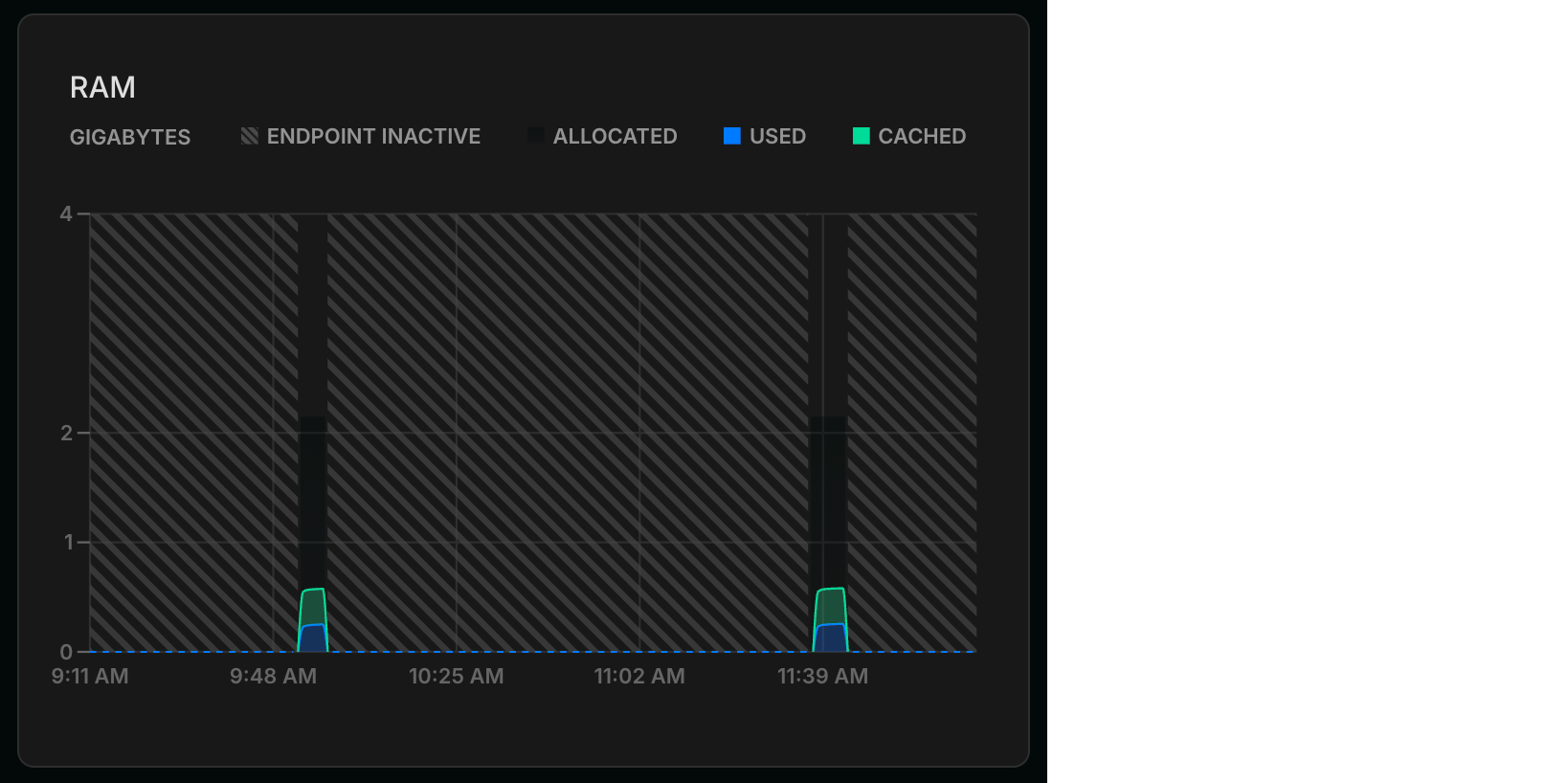
The values and plotted lines in your graphs will drop to `0` when your compute is inactive because a compute must be active to report data. These inactive periods are also shown as a diagonal line pattern in the graph, as shown here:

![monitoring graph diagonal pattern for inactive compute](/docs/introduction/monitor_inactive.png)
</Admonition>

## RAM

![Monitoring page RAM graph](/docs/introduction/monitor_ram.png)

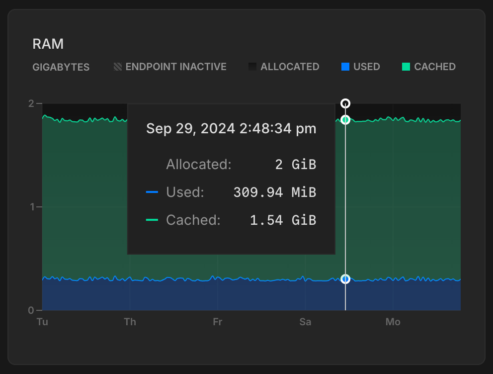
This graph shows allocated RAM and usage over time for the selected compute.

**ALLOCATED**: The amount of allocated RAM.

RAM is allocated according to the size of your compute or your [autoscaling](/docs/guides/autoscaling-guide) configuration, if applicable. For example, if your compute size is .25 CU (1 GB RAM), your allocated RAM is always 1 (GB). With autoscaling, allocated RAM increases and decreases as your compute size scales up and down in response to load. If [scale to zero](/docs/guides/scale-to-zero-guide) is enabled and your compute transitions to an idle state after a period of inactivity, allocated RAM drops to 0.

**Used**: The amount of RAM used.

The graph plots a line showing the amount of RAM used. If the line regularly reaches the maximum amount of allocated RAM, consider increasing your compute size to increase the amount of allocated RAM. To see the amount of RAM allocated for each Neon compute size, see [Compute size and autoscaling configuration](/docs/manage/computes#compute-size-and-autoscaling-configuration).

**Cached**: The amount of data cached in memory.

## CPU

![Monitoring page CPU graph](/docs/introduction/monitor_cpu.png)

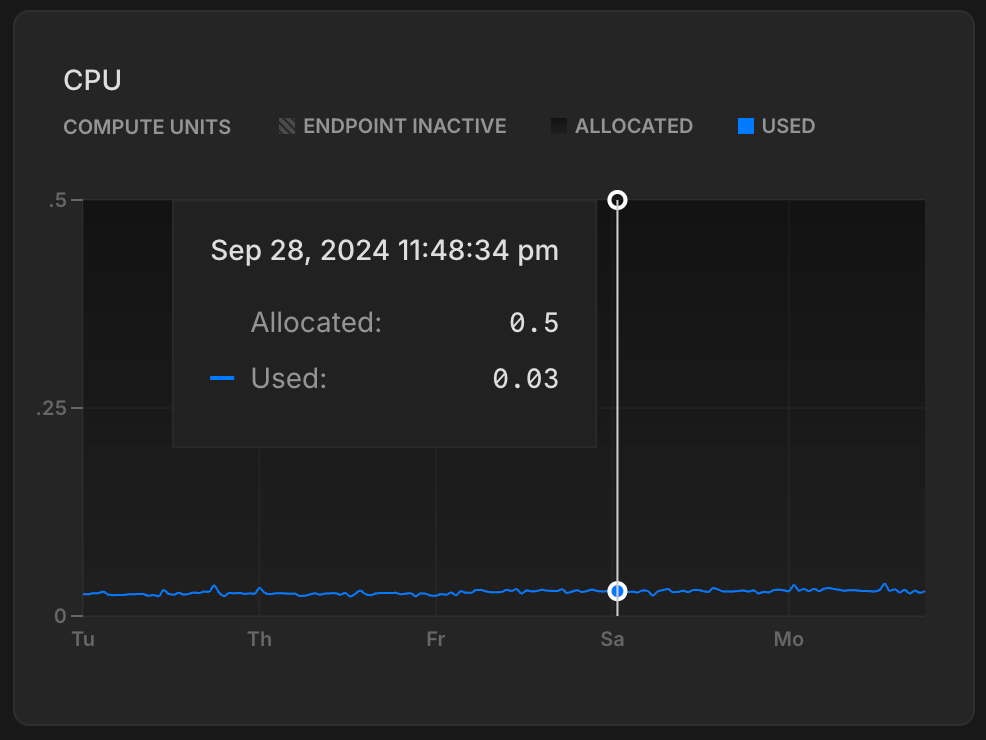
This graph shows the amount of allocated CPU and usage over time for the selected compute.

**ALLOCATED**: The amount of allocated CPU.

CPU is allocated according to the size of your compute or your [autoscaling](/docs/guides/autoscaling-guide) configuration, if applicable. For example, if your compute size is .25 CU (1 GB RAM), your allocated CPU scales proportionally. With autoscaling, allocated CPU increases and decreases as your compute size scales up and down in response to load. If [scale to zero](/docs/guides/scale-to-zero-guide) is enabled and your compute transitions to an idle state after a period of inactivity, allocated CPU drops to 0.

**Used**: The amount of CPU used, in [Compute Units (CU)](/docs/reference/glossary#compute-unit-cu).

If the plotted line regularly reaches the maximum amount of allocated CPU, consider increasing your compute size. To see the compute sizes available with Neon, see [Compute size and autoscaling configuration](/docs/manage/computes#compute-size-and-autoscaling-configuration).

## Postgres connections count

![Monitoring page connections graph](/docs/introduction/monitor_connections.png)

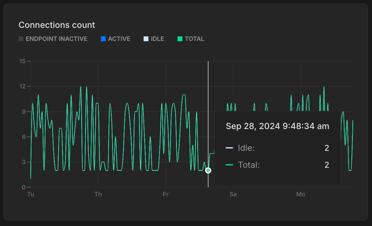
The **Postgres connections count** graph shows the number of idle connections, active connections, and the total number of connections directly to your Postgres database over time for the selected compute. These are the actual connections on the Postgres server itself.

**ACTIVE**: The number of active connections for the selected compute.

Monitoring active connections can help you understand your database workload at any given time. If the number of active connections is consistently high, it might indicate that your database is under heavy load, which could lead to performance issues such as slow query response times. See [Connections](/docs/postgresql/query-reference#connections) for related SQL queries.

**IDLE**: The number of idle connections for the selected compute.

Idle connections are those that are open but not currently being used. While a few idle connections are generally harmless, a large number of idle connections can consume unnecessary resources, leaving less room for active connections and potentially affecting performance. Identifying and closing unnecessary idle connections can help free up resources. See [Find long-running or idle connections](/docs/postgresql/query-reference#find-long-running-or-idle-connections).

**TOTAL**: The sum of active and idle connections for the selected compute.

**MAX**: The maximum number of simultaneous connections allowed for your compute size.

The MAX line helps you visualize how close you are to reaching your connection limit. When your TOTAL connections approach the MAX line, you may want to consider:

- Increasing your compute size to allow for more connections
- Implementing [connection pooling](/docs/connect/connection-pooling), which supports up to 10,000 simultaneous connections
- Optimizing your application's connection management

The connection limit (defined by the Postgres `max_connections` setting) is set according to your Neon compute size configuration. For the connection limit for each Neon compute size, see [How to size your compute](/docs/manage/computes#how-to-size-your-compute).

<Admonition type="note">
If you're using [connection pooling](/docs/connect/connection-pooling), also monitor the [Pooler client connections](#pooler-client-connections) and [Pooler server connections](#pooler-server-connections) graphs. When using a pooled connection, the **Pooler server connections** represent the actual connections from PgBouncer to Postgres, while this **Postgres connections count** graph shows all direct connections to Postgres (including those from the pooler and any direct connections).
</Admonition>

## Pooler client connections

![Pooler client connections graph](/docs/introduction/pooler_client_connections.png)

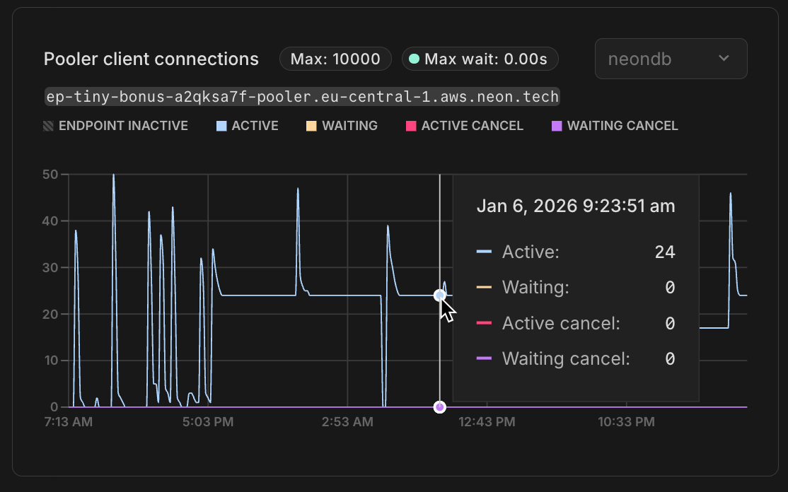
The **Pooler client connections** graph shows connections from your applications to Neon's PgBouncer connection pooler. This graph only displays data when you're using a [pooled connection string](/docs/connect/connection-pooling) (one that includes `-pooler` in the endpoint hostname).

PgBouncer supports up to 10,000 simultaneous client connections, which is significantly higher than the direct Postgres connection limit. The graph shows the following connection states:

**ACTIVE**: Client connections actively executing a query through the pooler.

These are connections that currently have an active query running. A high number of active connections indicates your application is actively using the database.

**WAITING**: Client connections waiting for an available server connection from the pool.

When all available server connections (connections from PgBouncer to Postgres) are in use, additional client requests must wait in a queue. If you consistently see a high number of waiting connections, it may indicate:

- Your workload requires more server connections than your current `default_pool_size` allows
- Long-running queries are holding server connections
- Your compute size may need to be increased to support more concurrent server connections

The graph also displays **Max wait**, which shows the maximum time (in seconds) that any client connection has been waiting for an available server connection. A consistently high max wait time indicates that clients are experiencing delays in getting database access, which could impact application performance

**ACTIVE CANCEL** and **WAITING CANCEL**: Connections in the process of being cancelled.

These represent client connections where a cancellation request has been issued (for example, when a user cancels a query).

<Admonition type="tip">
Connection pooling works by allowing many client connections to share a smaller pool of actual Postgres connections. While you can have thousands of client connections, they share a limited number of server connections determined by PgBouncer's `default_pool_size` setting. For more details, see [Connection pooling](/docs/connect/connection-pooling).
</Admonition>

## Pooler server connections

![Pooler server connections graph](/docs/introduction/pooler_server_connections.png)

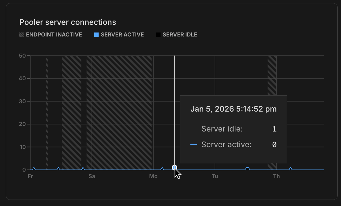
The **Pooler server connections** graph shows connections from Neon's PgBouncer pooler to your Postgres database. This graph only displays data when you're using a [pooled connection string](/docs/connect/connection-pooling) (one that includes `-pooler` in the endpoint hostname).

These server connections are shared by all client connections to the pooler, enabling thousands of clients to efficiently share a smaller pool of Postgres connections. The graph shows the following states:

**SERVER ACTIVE**: Server connections currently serving client queries.

These are the pooler's connections to Postgres that are actively processing queries from clients. This number represents the actual concurrent queries being executed on your Postgres database through the pooler.

**SERVER IDLE**: Server connections in the pool that are available but not currently in use.

PgBouncer maintains these idle connections in the pool so they're ready to handle new client requests without the overhead of establishing new connections. In transaction pooling mode (which Neon uses), connections are returned to the idle state as soon as a transaction completes.

The total number of server connections (active + idle) is limited by PgBouncer's `default_pool_size` setting, which is set to 0.9 × your compute's `max_connections`. For example:

- A 1 CU compute with `max_connections=450` can have up to 405 pooler server connections
- A 2 CU compute with `max_connections=901` can have up to 810 pooler server connections

<Admonition type="note">

The **Pooler server connections** count is a subset of what you see in the [Postgres connections count](#postgres-connections-count) graph. The Postgres connections count shows all connections to Postgres, including those from the pooler plus any direct (non-pooled) connections. To understand your complete connection picture when using pooling:

- **Pooler client connections**: Shows how many applications/clients are connected to the pooler
- **Pooler server connections**: Shows how many connections the pooler is using to Postgres (limited by `default_pool_size`)
- **Postgres connections count**: Shows all connections to Postgres (pooler connections + direct connections)

</Admonition>

## Database size

![Monitoring page database size graph](/docs/introduction/monitor_data_size.png)

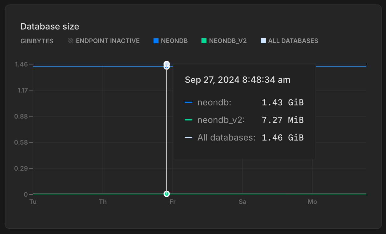
The **Database size** graph shows the logical data size (the size of your actual data) for the named database and the total size for all user-created databases (**All Databases**) on the selected branch. The **All Databases** metric is only shown when there is more than one database on the selected branch.

<Admonition type="important">
Database size metrics are only displayed while your compute is active. When your compute is idle, database size values are not reported, and the **Database size** graph shows zero even though data may be present.
</Admonition>

## Deadlocks

![Monitoring page deadlocks graph](/docs/introduction/monitor_deadlocks.png)

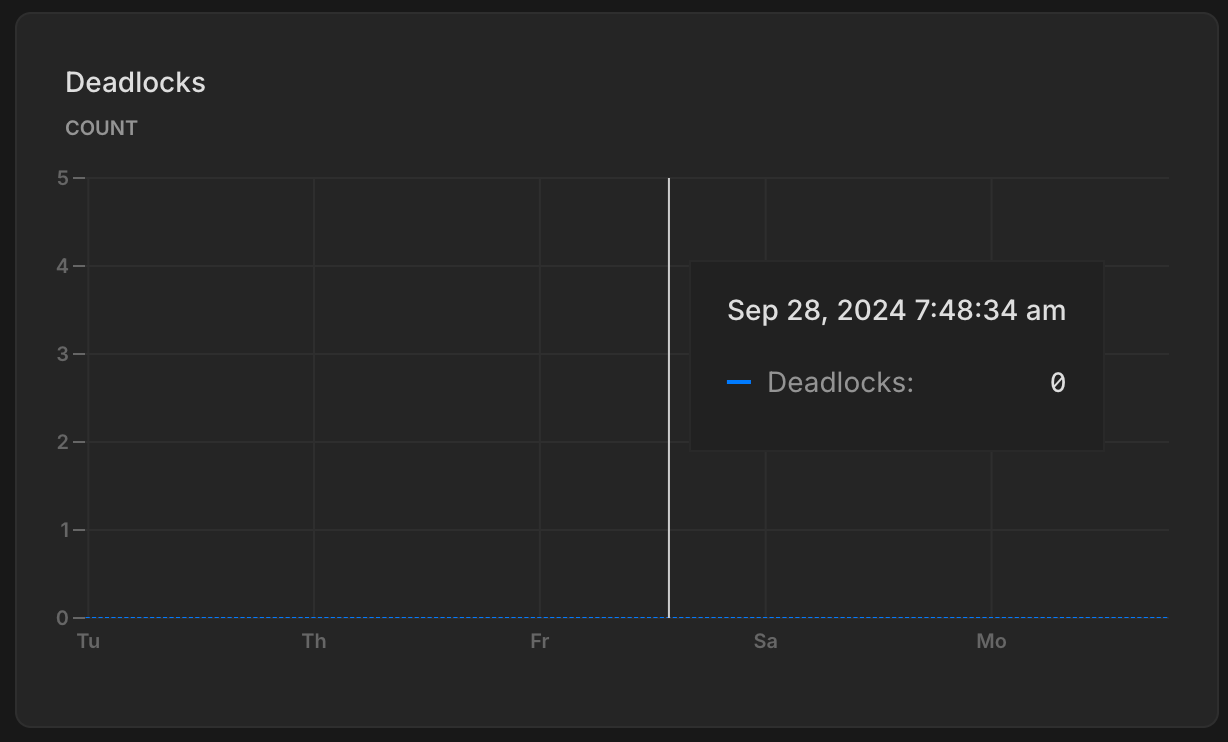
The **Deadlocks** graph shows a count of deadlocks over time for the named database on the selected branch. The named database is always the oldest database on the selected branch.

Deadlocks occur in a database when two or more transactions simultaneously block each other by holding onto resources the other transactions need, creating a cycle of dependencies that prevent any of the transactions from proceeding, potentially leading to performance issues or application errors. For lock-related queries you can use to investigate deadlocks, see [Performance tuning](/docs/postgresql/query-reference#performance-tuning). To learn more about deadlocks in Postgres, see [Deadlocks](https://www.postgresql.org/docs/current/explicit-locking.html).

## Rows

![Monitoring page rows graph](/docs/introduction/monitor_rows.png)

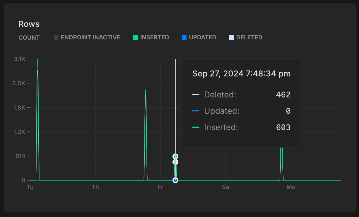
The **Rows** graph shows the number of rows deleted, updated, and inserted over time for the named database on the selected branch. The named database is always the oldest database on the selected branch. Row metrics are reset to zero whenever your compute restarts.

Tracking rows inserted, updated, and deleted over time provides insights into your database's activity patterns. You can use this data to identify trends or irregularities, such as insert spikes or an unusual number of deletions.

<Admonition type="note">
Row metrics only capture row-level changes (`INSERT`, `UPDATE`, `DELETE`, etc.) and exclude table-level operations such as `TRUNCATE`.
</Admonition>

## Replication delay bytes

![Replication delay bytes](/docs/introduction/rep_delay_bytes.png)

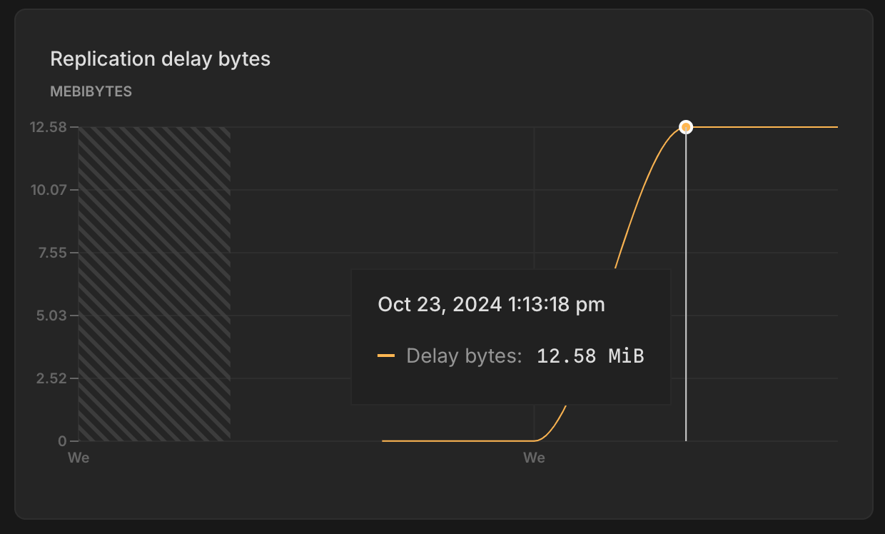
The **Replication delay bytes** graph shows the total size, in bytes, of the data that has been sent from the primary compute but has not yet been applied on the replica. A larger value indicates a higher backlog of data waiting to be replicated, which may suggest issues with replication throughput or resource availability on the replica. This graph is only visible when selecting a **Replica** compute from the **Compute** drop-down menu.

## Replication delay seconds

![Replication delay seconds](/docs/introduction/rep_delay_seconds.png)

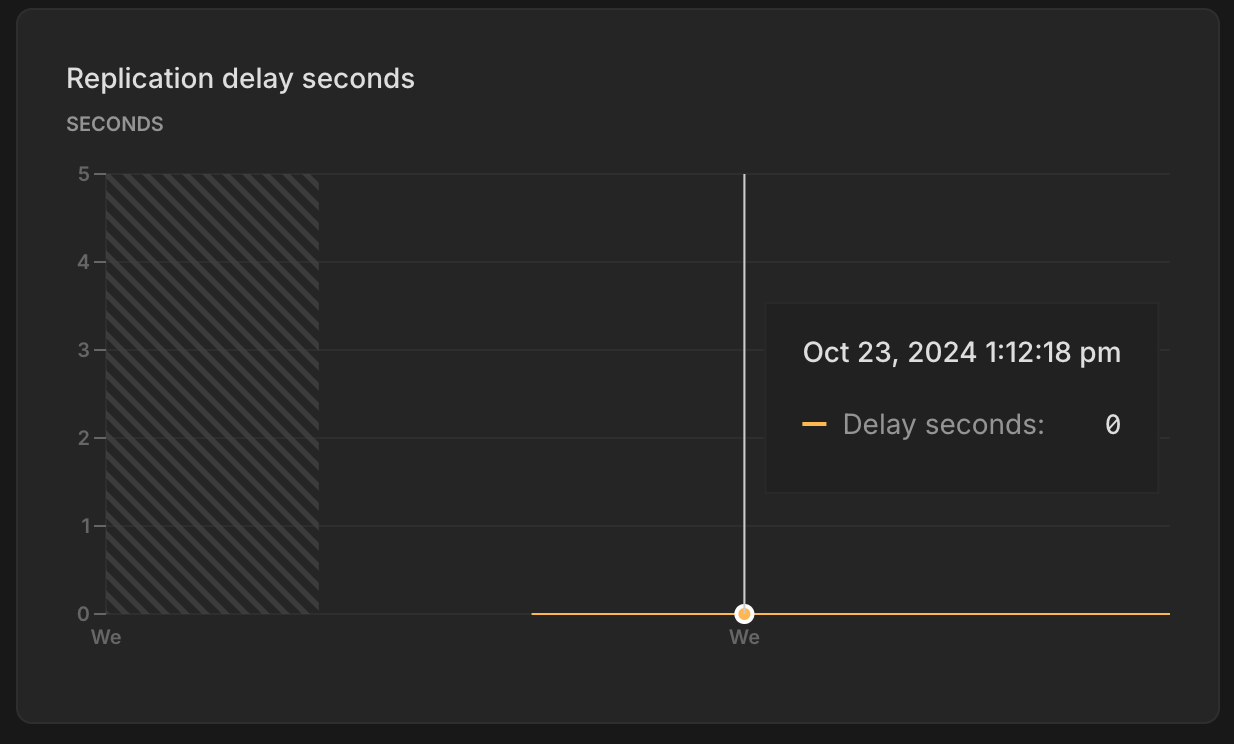
The **Replication delay seconds** graph shows the time delay, in seconds, between the last transaction committed on the primary compute and the application of that transaction on the replica. A higher value suggests that the replica is behind the primary, potentially due to network latency, high replication load, or resource constraints on the replica. This graph is only visible when selecting a **Replica** compute from the **Compute** drop-down menu.

## Local file cache hit rate

![local file cache hit rate graph](/docs/introduction/local_file_cache_hit_rate.png)

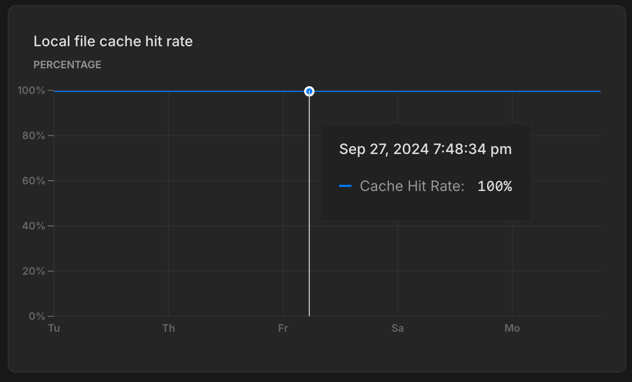
The **Local file cache hit rate** graph shows the percentage of read requests served from Neon's Local File Cache (LFC).
Queries not served from either Postgres shared buffers or the Local File Cache retrieve data from storage, which is more costly and can result in slower query performance. To learn more about how Neon caches data and how the LFC works with Postgres shared buffers, see [What is the Local File Cache?](/docs/extensions/neon#what-is-the-local-file-cache)

## Working set size

![working set size graph](/docs/introduction/working_set_size.png)

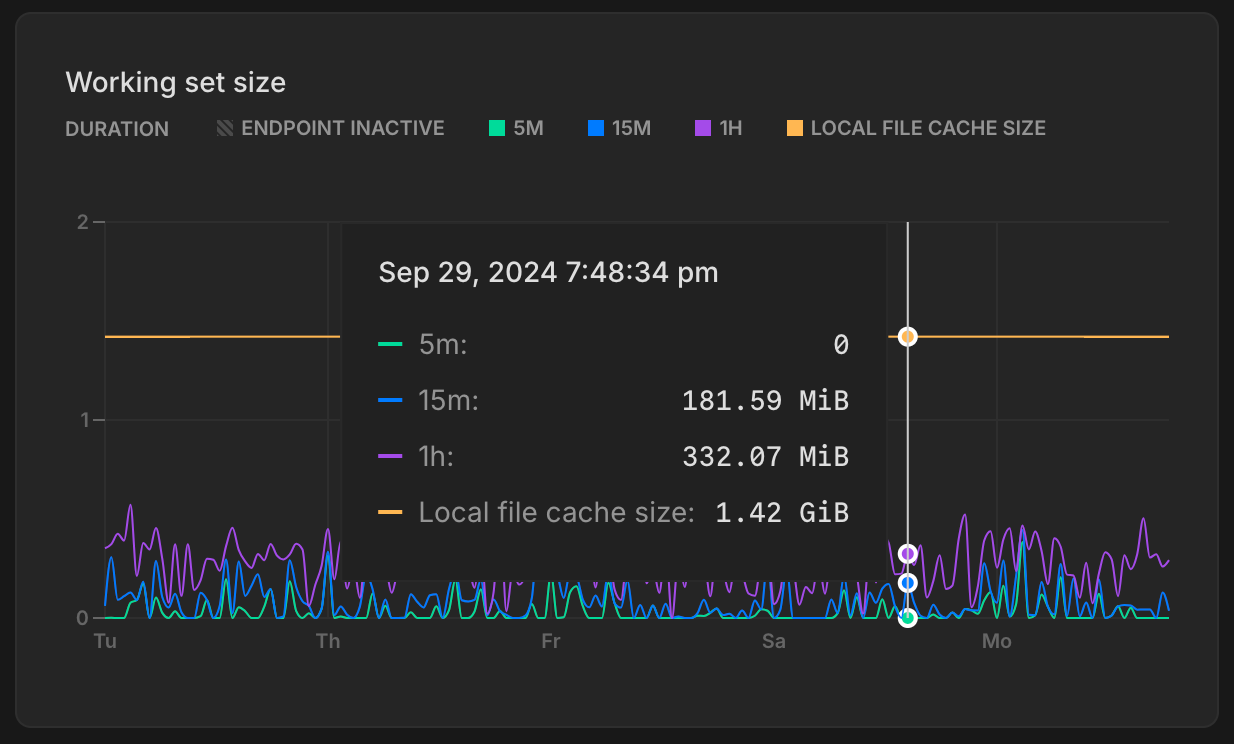
Your working set is the size of the distinct set of Postgres pages (relation data and indexes) accessed in a given time interval - to optimize for performance and consistent latency it is recommended to size your compute so that the working set fits into Neon's [Local File Cache (LFC)](/docs/extensions/neon#what-is-the-local-file-cache) for quick access.

The **Working set size** graph visualizes the amount of data accessed—calculated as unique pages accessed × page size—over a given interval. Here's how to interpret the graph:

- **5m** (5 minutes): This line shows the data accessed in the last 5 minutes.
- **15m** (15 minutes): Similar to the 5-minute window, this metric tracks the data accessed in the last 15 minutes.
- **1h** (1 hour): This line represents the data accessed in the last hour.
- **Local file cache size**: This is the size of the LFC, which is determined by the size of your compute. Larger computes have larger caches. For cache sizes, see [How to size your compute](/docs/manage/computes#how-to-size-your-compute).
  For optimal performance the local file cache should be larger than your working set size for a given time interval.
  If your working set size is larger than the LFC size it is recommended to increase the maximum size of the compute to improve the LFC hit rate and achieve good performance.

If your workload pattern doesn't change much over time it is recommended to compare the 1h time interval working set size with the LFC size and make sure that working set size is smaller than LFC size.